LightDock Basics
- 1. Introduction
- 2. Setup a simulation
- 3. Run a simulation
- 4. Generate models
- 5. Clustering
- 6. Summary
- 7. References
1. Introduction
1.1. What is LightDock?
LightDock is a protein-protein, protein-peptide and protein-DNA docking protocol based on the Glowworm Swarm Optimization (GSO) algorithm. In summary, LightDock is:
-
Ab initio protocol, which means that only requires the 3D coordinates of the structural partners for predicting protein-protein, protein-peptide or protein-DNA complexes.
-
Additional information (coming from experiments or bioinformatics predictions) in the form of residue restraints may be included during the docking calculations. The protocol is capable of taking into account this information in both receptor and/or ligand partners.
-
It is capable of modeling protein-protein, protein-peptide and protein-DNA interactions in rigid-body fashion or modeling backbone flexibility using Anisotropic Network Model (ANM). If ANM mode is activated, LightDock calculates the Ca-Ca ANM model using the awesome ProDy Python library. By default, the first 10 non-trivial normal modes are calculated for both receptor and ligand (in every residue backbone and further extended to the side-chains). See Prody ANM documentation for an example. The number of non-trivial normal modes can be tuned by the user.
-
Customizable by the user. LightDock is not only a protocol, but a framework for testing and developing custom scoring functions. The GSO optimization algorithm is agnostic of the force-field used, so in theory LightDock is capable of minimizing the docking energies in any force-field given by the user.
-
Prepared to scale in HPC architectures. LightDock nature is embarrassingly parallel as each swarm is treated as an independent simulation. This property makes LightDock to scale up to a number of CPU cores equal to the number of swarms simulated. Two implementations are given: 1) multiprocessing (by default) and 2) MPI (using mpi4py library, not installed by default).
-
It is possible to use several scoring functions during the minimization. Instead of specifying a single scoring function, a file containing the weight and the name of the scoring function can be given as an input. LightDock will combine the different scoring functions as a linear combination of their value multiplied by the weight specified in the file.
1.2. Swarms
In LightDock, the receptor molecule is kept fixed (despite atoms could move if ANM mode is enabled). Over its surface, a set of points is calculated. Each of these points is a swarm center which represents an independent simulation. For example, for complex 1PPE, 185 swarms are automatically calculated:
1.3. Glowworms
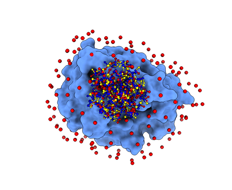
For each of these swarm centers, a given number N of glowworms, the algorithm agents, are disposed in a random way (if residue restraints are not specified). Every glowworm represents a possible ligand conformation. In the following figure two sets of 200 glowworms are displayed in two selected swarms:
More in detail, each glowworm is represented as a 3D-axis object in its center of mass and oriented as the actual 3D-axis orientation:
1.4. Optimization
LightDock, based on the GSO algorithm, will optimize the poses according to the amount of luciferin emitted (score). Poses will evolve in translational, rotational and ANM spaces towards better energetical regions.
In the video below, you can see how 300 initial glowworms poses (x, y, z) from a unique swarm evolve during an extended LightDock simulation (200 steps).
2. Setup a simulation
The first step of the LightDock protocol is setup. If you execute the lightdock3_setup.py command, several options will be displayed:
usage: lightdock3_setup [-h] [-s SWARMS] [-g GLOWWORMS] [--seed_points STARTING_POINTS_SEED] [--noxt]
                        [--noh] [--now] [--verbose_parser] [-anm] [--seed_anm ANM_SEED]
                        [--anm_rec_rmsd ANM_REC_RMSD] [--anm_lig_rmsd ANM_LIG_RMSD] [-ar ANM_REC]
                        [-al ANM_LIG] [-r restraints] [-membrane] [-transmembrane] [-sp]
                        [-sd SURFACE_DENSITY] [-sr SWARM_RADIUS] [-flip] [-fd FIXED_DISTANCE]
                        [-spr SWARMS_PER_RESTRAINT] [--ds] [-V]
                        receptor_pdb_file ligand_pdb_file
lightdock3_setup: error: the following arguments are required: receptor_pdb_file, ligand_pdb_file
The mandatory arguments (not enclosed by [ and ]) are:
- receptor_pdb_file: the file containing the receptor structure in PDB format
- ligand_pdb_file: the file containing the ligand structure in PDB format
Below, there is a description of the rest of accepted parameters by lightdock3_setup.py:
-s: the number of swarms of the simulations, if not provided by the user, automatically calculated depending on receptor surface area and shape-g: the number or glowworms for each swarm, if not provided by the user, 200 by defualt--seed_pointsSTARTING_POINTS_SEED: An integer can be specified as the seed used in the random number generator of the initial random poses of the ligand.--noxt: If this option is enabled, LightDock ignores OXT atoms. This is useful for several scoring functions which don’t understand this special type of atom.--noh: If this option is enabled, LightDock ignores hydrogen atoms. This is relevant fordfire,fastdfireordfire2scoring functions (among others). Only removes atoms starting withHcharacter, thus not recognizing types such as1H, etc.--now: If this option is enabled, crystal waters will be removed.--verbose_parser: If this option is enabled, LightDock will output in a verbose mode the atoms ignored when parsing PDB structures.--anm: If this option is enabled, the ANM mode is activated and backbone flexibility is modeled using ANM (via ProDy).--seed_anmANM_SEED: An integer can be specified as the seed used in the random number generator of ANM normal modes extents.-arANM_REC: The number of non-trivial normal modes calculated for the receptor in the ANM mode.-alANM_LIG: The number of non-trivial normal modes calculated for the ligand in the ANM mode.--anm_rec_rmsdANM_REC_RMSD: the maximum RMSD between generated ANM conformers and initial structure of the receptor. By default is 0.5Å.--anm_lig_rmsdANM_LIG_RMSD: the maximum RMSD between generated ANM conformers and initial structure of the ligand. By default is 0.5Å.-r, -rstrestraints_file: Ifrestraints_fileis provided, residue restraints will be considered during the setup and the simulation. See2.2. Residue Restraintssection for more information.-membrane: When enabled, this flag considers the receptor partner is aligned to the Z-axis and filters out swarms which would not be compatible with a trans-membrane domain. To do so, it makes use of the residues provided as receptor restraints.-transmembrane: When enabled, this flag considers the receptor partner is aligned to the Z-axis and filters out swarms which would not be inside the membrane.-sp: If enabled (False by default), writes in theinitfolder debugging extra files.-sdSURFACE_DENSITY: Controls the automatic calculation of swarms over the receptor surface. It is expressed as swarms/Å2-srSWARM_RADIUS: Controls the swarm size for creating the starting ligand poses. Radius is expressed in Å (Angstroms).-flip: Activates the 180° flip of 50% of starting poses when using restraints. This might help to capture symmetric binding interfaces.-fdFIXED_DISTANCE: Places swarms at a (approximated) fixed distance given by the user instead of using the ligand minimum radii. FIXED_DISTANCE is in Å.-sprSWARMS_PER_RESTRAINT: By default, a maximum of 20 swarms are kept by restraint to ensure a good sampling around provided residue-restraints. User might increase this to generate more swarms per restraint.--ds: Enables the dense sampling mode. This mode generates a massive number of swarms (see below):
2.1. Results of the setup
After the execution of the lightdock3_setup.py command, several files and directories will be generated in the root of your docking project:
init: A directory containing initialization data, see below:swarm_centers.pdb: A file in PDB format containing dummy atoms which coordinates correspond to a swarm center.initial_positions_X.dat: One file like this for each swarm (whereXindicates the id of the swarm), containing the translation, quaternion and normal modes extents (if ANM is activated) for each of the glowworms in this swarm.starting_positions_X.pdb: Same as before, but a PDB file with the glowworm translation vector expressed as a dummy atom (only ifspis enabled).starting_poses_X.bild: Same as before, but this time every glowworm pose in rotational space is expressed as a BILD 3D object which can be read by UCSF Chimera (only ifspis enabled). More information about the format can be found here.
swarm_0, ..., swarm_(N-1): For each of theNswarms specified by the-sargument or calculated automatically (by default), a directory is created. Note that the first directory is calledswarm_0and notswarm_1.setup.json: A file with a summary of the setup step in JSON format. This file will be necessary for running the simulation in the next step.lightdock_*.pdb: LightDock parses the input PDB structures and creates two new PDB files, one for the receptor and one for the ligand where the molecules have been centered to the origin of coordinates.*.xyz.npy: Two files with this extension, one for the receptor and one for the ligand, which contains information about the minimum ellipsoid containing each of the structures in NumPy format.lightdock_rec.nm.npyandlightdock_lig.nm.npy: If ANM is enabled, two files are created containing the normal modes information calculated by the ProDy library.*mask.npy: If ANM is enabled, two extra files are created containing a boolean NumPy array for the atoms of receptor and ligand to be used on ANM deformation.
2.2. Residue Restraints
Residue restraints on both receptor and/or ligand have been implemented. This feature works in the following way:
From a restraints_file file containing the following information:
R A.SER.150
R A.TYR.151 P
L B.LYS.2
L B.ARG.3 P
Where R means for Receptor and L means for Ligand, and then the rest of the line is a residue identifier in the format Chain.Residue_Name.Residue_Number[.Residue_Insertion] in the original PDB file numeration. Note that residue insertion codes are supported (for example, on using antibody-antigen systems with Chothia antibody numbering).
A P label in the end indicates this restraint is passive in contrast to active (no label).
We do not recommend to use passive residue restraints unless you understand completely their implications.
For each residue restraint specified for the receptor, only the closest swarms are considered during lightdock3_setup.py. At the moment, only the 10 closest swarms for each residue are considered. If some of the swarms overlap, then only one copy of that swarm is used. If no residue restraints at ligand level are specified, random orientations for the ligand molecule will be generated. On the other hand, if residue restraints on the ligand level have been defined, lightdock3_setup.py will find random {receptor residue restraint, ligand residue restraint} pairs (only considering the closest receptor residue restraints to the given swarm) and it will orient the given ligand residue restraint towards receptor residue restraint. With this mechanism, the algorithm is biased towards correct orientations of the ligand molecule.
Then, the simulation will try to optimize both energy and restraints satisfied taking into account only active residues.
Once the simulation has ended, the script lgd_filter_restraints.py can be used in order to remove predictions which do not satisfy the provided restraints provided a certain threshold.
2.3. Tips and tricks
-
As a general rule of thumb, the receptor structure is the bigger molecule and the ligand the smaller. For this concept of size, the metric used is the longest diameter of the minimum ellipsoid containing the molecule. A script called
lgd_calculate_diameter.pycan be found in$LIGHTDOCK_HOME/bin/path in order to calculate an approximation of that metric. -
If the
initdirectory exists,lightdock3_setup.pymakes use of the information contained in that directory. -
The file
setup.jsonis intended for reproducibility of the results, but not to be modified by the user. -
Passive residue restraints are used only to filter (receptor) or bias the initial orientations (ligand), but not considered in the scoring function.
3. Run a simulation
3.1. Parameters
In order to run a LightDock simulation, the lightdock3.py command has to be executed. If executed without arguments, a list of accepted options is displayed:
usage: lightdock3 [-h] [-f configuration_file] [-s SCORING_FUNCTION] [-sg GSO_SEED] [-t TRANSLATION_STEP]
                  [-r ROTATION_STEP] [-V] [-c CORES] [--profile] [-mpi] [-ns NMODES_STEP] [-min] [--listscoring]
                  [-l SWARM_LIST [SWARM_LIST ...]]
                  setup_file steps
lightdock3: error: the following arguments are required: setup_file, steps
The simplest way to execute a LightDock simulation is:
lightdock3.py setup.json 10
The first parameter is the configuration file generated on the setup step, the second is the number of steps of the simulation.
The rest of possible arguments which lightdock3.py accepts is:
-fconfiguration_file: This is a special file containing the different parameters of the GSO algorithm. By default, this is not necessary to change, but advanced users might change some of the values. Here it is an example of the content of this file:
##
#
# GlowWorm configuration file - algorithm parameters
#
##

[GSO]

# Rho
rho = 0.4

# Gamma
gamma = 0.6

# Initial Luciferin
initialLuciferin = 5.0

# Initial glowworm vision range (in A)
initialVisionRange = 15.0

# Max vision range (in A)
maximumVisionRange = 40.0

# Beta
beta = 0.16

# Max number of neighbors
maximumNeighbors = 5
These are the parameters used in the LightDock publication, many of them inherited from the original GSO publication. Please refer to the Kaipa, Krishnanand N. and Ghose, Debasish for more details.
-sSCORING_FUNCTION: Probably one of the most important parameters of the simulation. The user is able to change the default scoring function (DFIRE, fast C implementationfastdfire) using this flag. A name of a scoring function or a file containing the name and weight of multiple scoring functions are accepted. See section 3.2 for a complete list of accepted scoring functions and how to combine them.-cCORES: By default, LightDock makes use of the total number of available CPU cores on the hardware to run the simulation, but a different number of CPU cores can be specified via this option.-mpi: If this flag is activated, LightDock will make use of theMPI4pylibrary in order to spread to different nodes.--profile: This is an experimental flag and it is intended for profiling computation time and memory used by LightDock.-sgGSO_SEED: It is the integer used as a seed for the random number generator in charge of running the simulation. Different seeds will incur in different simulation outputs.-tTRANSLATION_STEP: When the translation part of the optimization vector is interpolated, this parameter controls the interpolation point. By default is set to 0.5.-rROTATION_STEP: When the rotation part of the optimization vector is interpolated (using quaternion SLERP), this parameter controls the interpolation point. By default is set to 0.5.-nsNMODES_STEP: When the ANM normal modes extent part of the optimization vector is interpolated, this parameter controls the interpolation point. By default is set to 0.5.-min: If this option is enabled, a local minimization of the best glowworm in terms of scoring is performed for each step, at each swarm. The algorithm used is the Powell (fmin_powell) implementation from thescipy.optimizelibrary. Optimization also includes ANM space (together with translation and rotational spaces) if-anmis enabled in the simulation.--listscoring: shows the scoring functions available.-lSWARM_LIST [SWARM_LIST …]: Only simulate the swarm IDs specified by this list. For example, to simulate only swarm 0:-l 0.-V: displays the LightDock version.
3.2. Available scoring functions
The complete list of scoring functions implemented in LightDock is:
cpydock: Implementation in C of the pyDock scoring function (also known as pyDockLite).dfire: Implementation of the DFIRE scoring function in Cython.fastdfire: Implementation of the DFIRE scoring function using the Python C-API, faster thandfire.dfire2: Implementation of the DFIRE2 scoring function using the Python C-API, despite a Cython version is also included for demonstrational purposes.dna: Implementation of the pyDockDNA scoring function (no desolvation) and custom Van der Waals weight for protein-DNA docking. Implemented using the Python C-API.ddna: Implementation of the DDNA scoring function as described in C. Zhang, S. Liu, Q. Zhu, and Y. Zhou, A knowledge-based energy function for protein-ligand, protein-protein and protein-DNA complexes, J. Med. Chem. 48, 2325-2335 (2005).mj3h: Pairwise contact energies for 20 types of residues, Mj3h.pisa: A statistical potential from the Improving ranking of models for protein complexes with side chain modeling and atomic potentials publication.sd: An electrostatics and Van der Waals based scoring function as described in the SwarmDock publication, but using AMBER94 force-field charges and parameters.sipper: Intermolecular pairwise propensities of exposed residues, SIPPER.tobi: TOBI potentials scoring function.vdw: A truncated Van der Waals (Lennard-Jones potential) as described in the original pyDock publication.
3.2.1. Multiple scoring functions
Several scoring functions can be used simultaneously by LightDock during the minimization. Each glowworm in the simulation will count on a model for each different scoring function, thus physical memory could be a limit on the number of simultaneous scoring functions.
A file containing the name of the scoring function and its weight can be defined as this example:
cat scoring.conf

sipper 0.5
dfire 0.8
For each pose, the scoring would be in this example the linear combination of both functions:
Scoring = 0.5*SIPPER + 0.8*DFIRE
Please note that combined scoring functions have to be compatible in terms of atom types (they recognized the same) and it is possible for all of them to make use of ANM (if enabled).
3.3. Tips and tricks
All the available scoring functions can be found at the path $LIGHTDOCK_HOME/lightdock/scoring. Each scoring function has its own directory in the source code tree.
4. Generate models
Once the simulation has completed, the predicted models can be generated as PDB structure files. In order to do so, execute the lgd_generate_conformations.py command:
usage: conformer_conformations [-h] [--setup setup_file]
                               receptor_structure ligand_structure lightdock_output glowworms
conformer_conformations: error: the following arguments are required: receptor_structure, ligand_structure, lightdock_output, glowworms
For example, to generate the 10 models predicted in the step 5 in a swarm populated by 10 glowworms of the 2UUY example:
cd $LIGHTDOCK_HOME/examples/2UUY
cd swarm_0
lgd_generate_conformations.py ../2UUY_rec.pdb ../2UUY_lig.pdb gso_5.out 10
IMPORTANT: note that the structures used by this command are the originals used in the lightdock3_setup.py command.
IMPORTANT: if lgd_generate_conformations.py command fails, please try again providing --setup setup_file.
5. Clustering
Intra-swarm clustering is essential for the protocol and it is not an optional step. This is specially critical for removing very similar structures in the swarm which have converged to the same structure and would add noise to the final ranking if not removed by the clustering. For each swarm, you can execute the lgd_cluster_bsas.py command:
cd swarm_0
lgd_cluster_bsas.py gso_5.out
The output would be:
Reading CA from lightdock_3.pdb
Reading CA from lightdock_6.pdb
Reading CA from lightdock_0.pdb
Reading CA from lightdock_5.pdb
Reading CA from lightdock_9.pdb
Reading CA from lightdock_7.pdb
Reading CA from lightdock_2.pdb
Reading CA from lightdock_8.pdb
Reading CA from lightdock_1.pdb
Reading CA from lightdock_4.pdb
Glowworm 6 with pdb lightdock_6.pdb
RMSD between 3 and 6 is 7.562
New cluster 1
Glowworm 0 with pdb lightdock_0.pdb
RMSD between 3 and 0 is 7.757
RMSD between 6 and 0 is 9.089
New cluster 2
Glowworm 5 with pdb lightdock_5.pdb
RMSD between 3 and 5 is 6.856
RMSD between 6 and 5 is 8.706
RMSD between 0 and 5 is 4.665
New cluster 3
Glowworm 9 with pdb lightdock_9.pdb
RMSD between 3 and 9 is 3.683
Glowworm 9 goes into cluster 0
Glowworm 7 with pdb lightdock_7.pdb
RMSD between 3 and 7 is 6.830
RMSD between 6 and 7 is 7.673
RMSD between 0 and 7 is 6.709
RMSD between 5 and 7 is 4.561
New cluster 4
Glowworm 2 with pdb lightdock_2.pdb
RMSD between 3 and 2 is 7.346
RMSD between 6 and 2 is 9.084
RMSD between 0 and 2 is 7.646
RMSD between 5 and 2 is 7.772
RMSD between 7 and 2 is 9.414
New cluster 5
Glowworm 8 with pdb lightdock_8.pdb
RMSD between 3 and 8 is 7.980
RMSD between 6 and 8 is 5.623
RMSD between 0 and 8 is 8.147
RMSD between 5 and 8 is 8.182
RMSD between 7 and 8 is 7.451
RMSD between 2 and 8 is 8.337
New cluster 6
Glowworm 1 with pdb lightdock_1.pdb
RMSD between 3 and 1 is 5.530
RMSD between 6 and 1 is 9.025
RMSD between 0 and 1 is 6.481
RMSD between 5 and 1 is 6.954
RMSD between 7 and 1 is 7.928
RMSD between 2 and 1 is 3.114
Glowworm 1 goes into cluster 5
Glowworm 4 with pdb lightdock_4.pdb
RMSD between 3 and 4 is 9.306
RMSD between 6 and 4 is 7.367
RMSD between 0 and 4 is 8.225
RMSD between 5 and 4 is 9.455
RMSD between 7 and 4 is 8.641
RMSD between 2 and 4 is 9.509
RMSD between 8 and 4 is 7.742
New cluster 7
{0: [3, 9], 1: [6], 2: [0], 3: [5], 4: [7], 5: [2, 1], 6: [8], 7: [4]}
A new file in CSV format is created with the clustering information:
cat cluster.repr

0:2: 9.87810:3:lightdock_3.pdb
1:1: 9.66368:6:lightdock_6.pdb
2:1: 7.52192:0:lightdock_0.pdb
3:1: 7.36888:5:lightdock_5.pdb
4:1: 6.46572:7:lightdock_7.pdb
5:2: 5.66227:2:lightdock_2.pdb
6:1: 5.03967:8:lightdock_8.pdb
7:1:-34.67761:4:lightdock_4.pdb
For each line, the information is:
cluster_id : population : best_scoring : glowworm_id : representative PDB structure
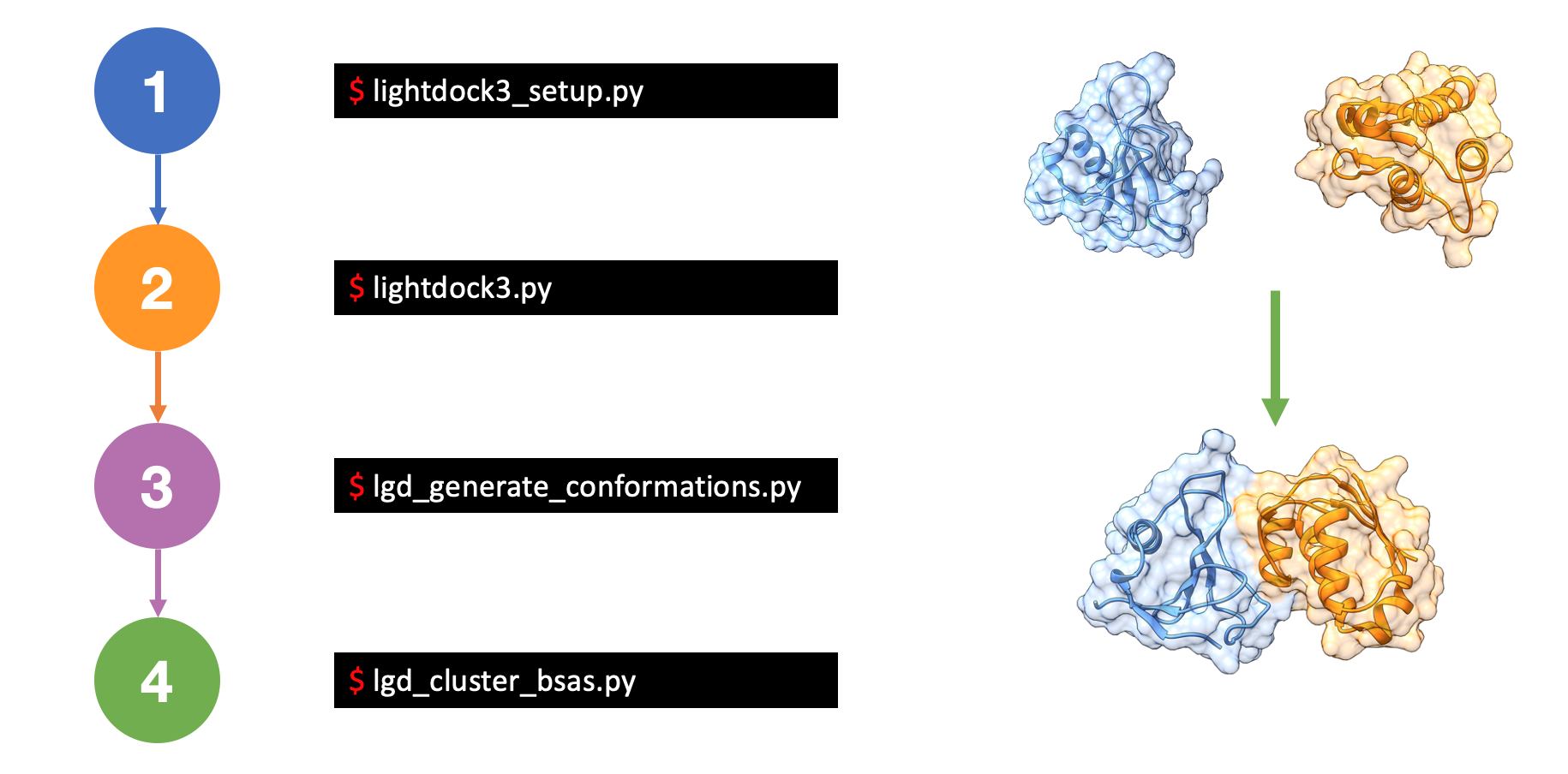
6. Summary
In summary, these are the main steps of any LightDock simulation:
7. References
For a more complete description of the algorithm as well as different tutorials, please refer to LightDock, or check the following references:
-
Integrative Modeling of Membrane-associated Protein Assemblies
Jorge Roel-Touris, Brian Jiménez-García & Alexandre M.J.J. Bonvin
Nat Commun 11, 6210 (2020); doi: https://doi.org/10.1038/s41467-020-20076-5 -
LightDock goes information-driven
Jorge Roel-Touris, Alexandre M.J.J. Bonvin and Brian Jiménez-García
Bioinformatics, Volume 36, Issue 3, 1 February 2020, Pages 950–952, doi: https://doi.org/10.1093/bioinformatics/btz642 -
LightDock: a new multi-scale approach to protein–protein docking
Brian Jiménez-García, Jorge Roel-Touris, Miguel Romero-Durana, Miquel Vidal, Daniel Jiménez-González and Juan Fernández-Recio
Bioinformatics, Volume 34, Issue 1, 1 January 2018, Pages 49–55, doi: https://doi.org/10.1093/bioinformatics/btx555