Protein-RNA docking prediction
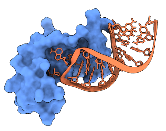
This is a complete example of the LightDock docking protocol to model the 1A1T protein-RNA complex.
This tutorial has been contributed by Lucas Goiriz Beltrán, and makes use of several additional Python scripts and LightDock hacks. Please note that protein-RNA docking is very experimental in LightDock.
You may contact Lucas Goiriz by email for doubts and insights about this tutorial and protocol.
1. Copying the data
Create a directory and copy the sample data provided.
mkdir 1a1t
cd 1a1t
curl -O https://raw.githubusercontent.com/lightdock/lightdock.github.io/master/tutorials/0.9.3/rna_docking/data/1A1T_A.pdb
curl -O https://raw.githubusercontent.com/lightdock/lightdock.github.io/master/tutorials/0.9.3/rna_docking/data/1A1T_B.pdb
2. Protonation
2.1. Protein
First of all, we need the protein partner to have the correct hydrogen atoms as parametrized in our dna scoring function (dna scoring function is based in the AMBER94 force-field).
Although this is a protein-RNA docking example, we will use the dna scoring function because the AMBER94 force-field also includes parameters for RNA residues.
To do it so, we will use the software reduce which can be downloaded from GitHub.
We remove the previous hydrogens and them rebuild them according to reduce.
reduce -Trim 1A1T_A.pdb > 1A1T_A_noh.pdb
reduce -BUILD 1A1T_A_noh.pdb > 1A1T_A_h.pdb
We have renumbered the atoms of the protein receptor partner using the PDB-Tools (web server or Python Package):
pdb_reatom 1A1T_A_h.pdb > protein.pdb
You can find this file already generated for you here: protein.pdb
2.2. RNA
We do the same as in previous section for the RNA partner (ligand):
reduce -Trim 1A1T_B.pdb > 1A1T_B_noh.pdb
reduce -BUILD 1A1T_B_noh.pdb > 1A1T_B_h.pdb
There are several problems we must address in order to continue:
- Hydrogen atoms produced by
reducefor nucleic acids are not 100% name-compatible with the AMBER94 force-field. - In addition,
reduceadds the extremal hydrogens (3’ and/or 5’ extremal hydrogens) to RNA, which causes conflicts with the AMBER94 force-field. - Finally, the AMBER94 force-field needs RNA residues to be labelled with an
Ras a prefix.
We have prepared three simple Python scripts:
- one to rename and/or remove incompatible atom types: reduce_to_amber.py
- one to remove the extremal hydrogens purge_prime_H.py
- one to add or remove the
Rtag for RNA residues: retag_rna.py
You must execute these scripts on the previous reduce output in the following order:
./retag_rna.py 1A1T_B_h.pdb rna_pre.pdb
./reduce_to_amber.py rna_pre.pdb rna_pre2.pdb
./purge_prime_H.py rna_pre2.pdb rna_tagged.pdb
This script is not covering at the moment all the non-compatible hydrogen atoms, but you can easily adapt it to your needs. For an exhaustive list of atoms supported by the dna scoring function check this file: amber.py
In order to obtain the final structure ready for LightDock, we must remove the R tags we added in the previous step. We can do so by employing retag_rna.py with the -r flag:
./retag_rna.py -r rna_tagged.pdb rna.pdb
Finally, we provide the RNA PDB structure ready for LightDock here: rna.pdb
4. Setup
First, we need to run the setup step. We will leave the number of swarms and glowworms by default, but we will enable the flexibility:
lightdock3_setup.py protein.pdb rna.pdb -anm
You will see an output similar to this:
@> ProDy is configured: verbosity='none'
[lightdock3_setup] INFO: Reading structure from protein.pdb PDB file...
[lightdock3_setup] INFO: 884 atoms, 55 residues read.
[lightdock3_setup] INFO: Reading structure from rna.pdb PDB file...
[lightdock3_setup] INFO: 650 atoms, 20 residues read.
[lightdock3_setup] INFO: Calculating reference points for receptor protein.pdb...
[lightdock3_setup] INFO: Reference points for receptor found, skipping
[lightdock3_setup] INFO: Done.
[lightdock3_setup] INFO: Calculating reference points for ligand rna.pdb...
[lightdock3_setup] INFO: Reference points for ligand found, skipping
[lightdock3_setup] INFO: Done.
[lightdock3_setup] INFO: Saving processed structure to PDB file...
[lightdock3_setup] INFO: Done.
[lightdock3_setup] INFO: Saving processed structure to PDB file...
[lightdock3_setup] INFO: Done.
[lightdock3_setup] INFO: Calculating ANM for receptor molecule...
[lightdock3_setup] INFO: 10 normal modes calculated
[lightdock3_setup] INFO: Calculating ANM for ligand molecule...
[lightdock3_setup] INFO: 10 normal modes calculated
[lightdock3_setup] INFO: Calculating starting positions...
[lightdock3_setup] INFO: Generated 102 positions files
[lightdock3_setup] INFO: Done.
[lightdock3_setup] INFO: Number of calculated swarms is 102
[lightdock3_setup] INFO: Preparing environment
[lightdock3_setup] INFO: Done.
[lightdock3_setup] INFO: LightDock setup OK
You will notice that the setup step produced a series of files. One of them is lightdock_rna.pdb, which contains the processed RNA ligand structure that LightDock is going to employ in the docking simulation.
Again, for the AMBER94 force field to work, we need to add the R tag to the RNA residues. We can do so by employing retag_rna.py again:
mv lightdock_rna.pdb lightdock_rna_untagged.pdb
./retag_rna.py lightdock_rna_untagged.pdb lightdock_rna.pdb
Now the simulation will run without issues.
5. Simulation
We can run this simulation in a local machine or in a HPC cluster. For the first option, simply run the following command.
lightdock3.py setup.json 100 -s dna -c 8
Where the flag -c 8 indicates LightDock to use 8 available cores. For this example we will run 100 steps of the protocol and using a scoring function with support for nucleic acids: -s dna.
To run a LightDock job on a HPC cluster, a Portable Batch System (PBS) file can be generated. This PBS file defines the commands and cluster resources used for the job. A PBS file is a plain-text file that can be easily edited with any UNIX editor.
For example, create a new submit_job.sh file containing:
#PBS -N LightDock-1A1T
#PBS -q medium
#PBS -l nodes=1:ppn=16
#PBS -S /bin/bash
#PBS -d ./
#PBS -e ./lightdock.err
#PBS -o ./lightdock.out

lightdock3.py setup.json 100 -s dna -c 16
This script tells the PBS queue manager to use 16 cores of a single node in a queue with name medium, with job name LigthDock-1A1T and with standard output to lightdock.out and error output redirected to lightdock.err.
To run this script you can do it as:
qsub < submit_job.sh
6. Clustering and Filtering
Once the simulation has finished (it takes around 6-7 min per 100 steps per swarm), we need to generate the structures of the predictions and cluster them per swarm.
For this step, it is essential that the file lightdock_rna.pdb does not have the RNA residue tag R. Since we have an untagged version of the file, called lightdock_rna_untagged.pdb, we don’t have to run retag_rna.py as renaming the files is sufficient:
mv lightdock_rna.pdb lightdock_rna_tagged.pdb
mv lightdock_rna_untagged.pdb lightdock_rna.pdb
Now we can proceed with generating the structures of the predictions and clustering them per swarm.
Here there is a PBS script to do all steps at once:
#PBS -N 1A1T-post
#PBS -q medium
#PBS -l nodes=1:ppn=8
#PBS -S /bin/bash
#PBS -d ./
#PBS -e ./postprocessing.err
#PBS -o ./postprocessing.out

### Calculate the number of swarms ###
s=`ls -d ./swarm_* | wc -l`
swarms=$((s-1))

### Create files for Ant-Thony ###
for i in $(seq 0 $swarms)
  do
    echo "cd swarm_${i}; lgd_generate_conformations.py ../protein.pdb ../rna.pdb  gso_100.out 200 > /dev/null 2> /dev/null;" >> generate_lightdock.list;
  done

for i in $(seq 0 $swarms)
  do
    echo "cd swarm_${i}; lgd_cluster_bsas.py gso_100.out > /dev/null 2> /dev/null;" >> cluster_lightdock.list;
  done

### Generate LightDock models ###
ant_thony.py -c 8 generate_lightdock.list;

### Clustering BSAS (rmsd) within swarm ###
ant_thony.py -c 8 cluster_lightdock.list;

### Generate ranking files ###
lgd_rank.py $s 100;
NOTE: You can also run the previous commands locally in a sequential way.
Once the post-processing is finished, we will have a summary file of the predicted structures, including several information such s the swarm and glowworm it comes from, the luciferin score, etc… We can take a look at it:
head solutions.list
Which will output something similar to this:
Swarm  Glowworm  ...  Luciferin  Neigh    VR  RMSD                PDB  Clashes  Scoring
    0        54  ...   88.78862      0  5.00  -1.0   lightdock_54.pdb        0   59.194
    0        57  ...  143.38735      0  0.40  -1.0   lightdock_57.pdb        0   97.943
    0        73  ...  125.13195      0  5.00  -1.0   lightdock_73.pdb        0   83.438
    0        78  ...   52.63139      2  5.00  -1.0   lightdock_78.pdb        0   36.038
    0        79  ...  201.78416      4  0.72  -1.0   lightdock_79.pdb        0  136.622
  ...       ...  ...        ...    ...   ...   ...                ...      ...      ...
  101       157  ...  167.36436      1  0.72  -1.0  lightdock_157.pdb        0  112.798
  101       165  ...  202.37440      2  5.00  -1.0  lightdock_165.pdb        0  135.225
  101       169  ...  -20.71950      1  5.00  -1.0  lightdock_169.pdb        0  -12.245
  101       183  ...  163.94394      2  1.80  -1.0  lightdock_183.pdb        0  111.157
  101       194  ...   88.41102      1  4.04  -1.0  lightdock_194.pdb        0   59.990
Note that the above output has been cut for the sake of readability.
We can sort this file by the Scoring variable and get the .pdb files of the top scoring structures. One way of doing this is by means of the get_top_structures.py Python script:
./get_top_structures.py solutions.list
This creates the top_structures directory with the top 10 scoring structures, prefixed by their order (being the 0 prefixed structure the best, and the 9 prefixed structure the worst).
We can compare the goodness of our docking simulation by aligning our best model with the crystal structure, by means of pymol’s align command. The output is something like this:
 Match: read scoring matrix.
 Match: assigning 77 x 75 pairwise scores.
 MatchAlign: aligning residues (77 vs 75)...
 MatchAlign: score 511.500
 ExecutiveAlign: 1429 atoms aligned.
 Executive: RMSD =    3.354 (1429 to 1429 atoms)
We provide for this example a complete simulation.tgz compressed file of the complete run.
7. References
For a more complete description of the algorithm as well as different tutorials, please refer to LightDock, or check the following references:
-
Integrative Modeling of Membrane-associated Protein Assemblies
Jorge Roel-Touris, Brian Jiménez-García & Alexandre M.J.J. Bonvin
Nat Commun 11, 6210 (2020); doi: https://doi.org/10.1038/s41467-020-20076-5 -
LightDock goes information-driven
Jorge Roel-Touris, Alexandre M.J.J. Bonvin and Brian Jiménez-García
Bioinformatics, Volume 36, Issue 3, 1 February 2020, Pages 950–952, doi: https://doi.org/10.1093/bioinformatics/btz642 -
LightDock: a new multi-scale approach to protein–protein docking
Brian Jiménez-García, Jorge Roel-Touris, Miguel Romero-Durana, Miquel Vidal, Daniel Jiménez-González and Juan Fernández-Recio
Bioinformatics, Volume 34, Issue 1, 1 January 2018, Pages 49–55, doi: https://doi.org/10.1093/bioinformatics/btx555