Protein-protein docking using residue restraints
- 1. Copying the data
- 2. Specifying residue restraints
- 3. Setup
- 4. Simulation
- 5. Clustering and Filtering
- 6. References
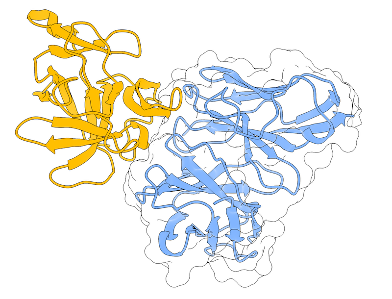
This is a complete example of the LightDock docking protocol to model the 4G6M protein complex with the use of residue restraints.
IMPORTANT Before starting with this tutorial, we advise you to follow the LightDock basics and simple docking tutorials.
1. Copying the data
Create a directory and copy the sample data provided.
mkdir test
cd test
curl -O https://raw.githubusercontent.com/lightdock/lightdock.github.io/master/tutorials/0.9.1/restraints/data/4G6M_rec.pdb
curl -O https://raw.githubusercontent.com/lightdock/lightdock.github.io/master/tutorials/0.9.1/restraints/data/4G6M_lig.pdb
2. Specifying residue restraints
LightDock is able to use information derived from either experimental information and/or bioinformatic predictions to drive the docking at several levels. This information is used in the form of residue restraints.
To do it so, we first need to create a restraints.list file with the following form:
R A.GLN.27
R A.SER.30
R A.TYR.32
...
L B.SER.68
L B.CYS.69
L B.VAL.70
...
Where the first column will indicate whether it is a receptor R or ligand L restraint, followed by CHAIN_ID.RESIDUE_NAME.RESIDUE_NUMBER[RESIDUE_INSERTION_CODE] (note RESIDUE_INSERTION_CODE is optional). In this case, LightDock will consider these residue restraints as active.
By contrast, if you want to define your residue restraints as passive, you should add an additional column with a P label.
R A.GLN.27 P
R A.SER.30 P
R A.TYR.32 P
...
L B.SER.68 P
L B.CYS.69 P
L B.VAL.70 P
...
NOTE For a detailed description of the exact implications of ACTIVE and PASSIVE restraints in LightDock, please refer to LightDock goes information-driven
For the sake of simplicity, we will use a list of residue restraints already formatted:
curl -O https://raw.githubusercontent.com/lightdock/lightdock.github.io/master/tutorials/0.9.1/restraints/data/restraints.list
3. Setup
First, we need to run the setup step. We will enable flexibility (-anm), exclude the terminal oxygens (--noxt) and all hydrogens (--noh) and water (--now) since those atoms are not parametrized in the fastdfire scoring function.
At this step, we need to also specify the residue restraints that will bias the docking simulation.
lightdock3_setup.py 4G6M_rec.pdb 4G6M_lig.pdb --noxt --noh --now -anm -rst restraints.list
You should see an output similar to this:
@> ProDy is configured: verbosity='info'
[lightdock_setup] INFO: Reading structure from 4G6M_rec.pdb PDB file...
[lightdock_setup] INFO: 1782 atoms, 230 residues read.
[lightdock_setup] INFO: Reading structure from 4G6M_lig.pdb PDB file...
[lightdock_setup] INFO: 1194 atoms, 149 residues read.
[lightdock_setup] INFO: Calculating reference points for receptor 4G6M_rec.pdb...
[lightdock_setup] INFO: Done.
[lightdock_setup] INFO: Calculating reference points for ligand 4G6M_lig.pdb...
[lightdock_setup] INFO: Done.
[lightdock_setup] INFO: Saving processed structure to PDB file...
[lightdock_setup] INFO: Done.
[lightdock_setup] INFO: Saving processed structure to PDB file...
[lightdock_setup] INFO: Done.
[lightdock_setup] INFO: 10 normal modes calculated
[lightdock_setup] INFO: 10 normal modes calculated
[lightdock_setup] INFO: Reading restraints from restraints.list
[lightdock_setup] INFO: Number of receptor restraints is: 20 (active), 0 (passive)
[lightdock_setup] INFO: Number of ligand restraints is: 21 (active), 0 (passive)
[lightdock_setup] INFO: Calculating starting positions...
[lightdock_setup] INFO: Generated 55 positions files
[lightdock_setup] INFO: Done.
[lightdock_setup] INFO: Number of swarms is 55 after applying restraints
[lightdock_setup] INFO: Preparing environment
[lightdock_setup] INFO: Done.
[lightdock_setup] INFO: LightDock setup OK
At first glance, we see that the default number of swarms (400) has been reduced to 55. This means that the sampling will be targeted towards a desired area of the receptor.
Moreover, since we have also specified residue restraints on the ligand, the initial glowworm conformations have been pre-oriented so that those residues will be facing the desired receptor’s region.
Please refer to the following picture for a graphical description of the setup:
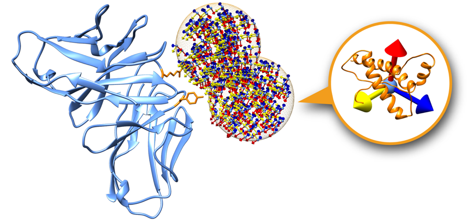
This is a representation of two swarms (orange mesh) over the surface of the 4G6M_rec.pdb structure (blue). In orange, two residues considered as restraints and therefore used to filter out the initial swarms prior the simulation. The initial orientations of the ligands within the swarms are represented using an orthogonal axis (x, y, z).
4. Simulation
We can run our simulation in a local machine or in a HPC cluster. For the first option, simply run the following command for simulating all 55 swarms:
lightdock3.py setup.json 100 -s fastdfire -c 8
Where the flag -c 8 indicates LightDock to use 8 available cores. For this example we will run 100 steps of the protocol and the C implementation of the DFIRE function -s fastdfire.
To run a LightDock job on a HPC cluster, a Portable Batch System (PBS) file can be generated. This PBS file defines the commands and cluster resources used for the job. A PBS file is a plain-text file that can be easily edited with any UNIX editor.
For example, create a submit_job.sh file containing:
#PBS -N LightDock-4G6M
#PBS -q medium
#PBS -l nodes=1:ppn=16
#PBS -S /bin/bash
#PBS -d ./
#PBS -e ./lightdock.err
#PBS -o ./lightdock.out

lightdock3.py setup.json 100 -s fastdfire -c 16
This script instructs the PBS queue manager to use 16 cores of a single node in a queue with name medium, with job name LigthDock-4G6M and with standard output to lightdock.out and error output redirected to lightdock.err.
To run this script you can do it as:
qsub < submit_job.sh
You may try to only simulate the first swarm (ID=0) with the following command:
lightdock3.py setup.json 100 -c 1 -l 0
5. Clustering and Filtering
Once the simulation has finished (it takes around 1-2 min per 10 steps per swarm), we need to cluster redundant predictions intra-swarm and filter out predictions which are compatible with the provided restraints during the setup step.
Attention! In order to get realistic simulations results it is critical to always cluster intra-swarm structures and to filter them for restraints compatibility.
5.1. Generating structures
We will generate the structures per swarm (200 glowworms per swarm in this example) required for the clustering and filtering steps.
This is a bash script which generates the predicted structures:
#!/bin/bash

CORES=8
s=`ls -d ./swarm_* | wc -l`
swarms=$((s-1))

### Create files for Ant-Thony ###
for i in $(seq 0 $swarms)
  do
    echo "cd swarm_${i}; lgd_generate_conformations.py ../4G6M_rec.pdb ../4G6M_lig.pdb  gso_100.out 200 > /dev/null 2> /dev/null;" >> generate_lightdock.list;
  done

### Generate LightDock models ###
ant_thony.py -c ${CORES} generate_lightdock.list;
5.2. Clustering structures intra-swarm
This is a bash script which clusters the different structures per swarm, already generated in previous section:
#!/bin/bash

CORES=8
s=`ls -d ./swarm_* | wc -l`
swarms=$((s-1))

### Create files for Ant-Thony ###
for i in $(seq 0 $swarms)
  do
    echo "cd swarm_${i}; lgd_cluster_bsas.py gso_100.out > /dev/null 2> /dev/null;" >> cluster_lightdock.list;
  done

### Cluster LightDock models ###
ant_thony.py -c ${CORES} cluster_lightdock.list;
5.3. Generating rank and filtering
Now you can create the best predictions rank by LightDock score:
lgd_rank.py $s 100;
And filter by a percentage of satisfied restraints (>40% in this example)
lgd_filter_restraints.py --cutoff 5.0 --fnat 0.4 rank_by_scoring.list restraints.list A B
5.4. Full protocol
Here there is a PBS script to do all previous steps at once:
#PBS -N 4G6M-anal
#PBS -q medium
#PBS -l nodes=1:ppn=8
#PBS -S /bin/bash
#PBS -d ./
#PBS -e ./analysis.err
#PBS -o ./analysis.out

CORES=8

### Calculate the number of swarms ###
s=`ls -d ./swarm_* | wc -l`
swarms=$((s-1))

### Create files for Ant-Thony ###
for i in $(seq 0 $swarms)
  do
    echo "cd swarm_${i}; lgd_generate_conformations.py ../4G6M_rec.pdb ../4G6M_lig.pdb  gso_100.out 200 > /dev/null 2> /dev/null;" >> generate_lightdock.list;
  done

for i in $(seq 0 $swarms)
  do
    echo "cd swarm_${i}; lgd_cluster_bsas.py gso_100.out > /dev/null 2> /dev/null;" >> cluster_lightdock.list;
  done


### Generate LightDock models ###
ant_thony.py -c ${CORES} generate_lightdock.list;


### Clustering BSAS (rmsd) within swarm ###
ant_thony.py -c ${CORES} cluster_lightdock.list;


### Generate ranking files for filtering ###
lgd_rank.py $s 100;


### Filtering models by >40% of satisfied restraints ###
lgd_filter_restraints.py --cutoff 5.0 --fnat 0.4 rank_by_scoring.list restraints.list A B > /dev/null 2> /dev/null;
Once the clustering and filtering steps have finished, a new directory called filtered has been created, which contains any predicted structure which satisfies our 40% filtering. Inside of this directory, there is a file with the ranking of these structures by LightDock DFIRE (fastdfire) score (the more positive the better) called rank_filtered.list.
6. References
For a more complete description of the algorithm as well as different tutorials, please refer to LightDock, or check the following references:
-
Integrative Modeling of Membrane-associated Protein Assemblies
Jorge Roel-Touris, Brian Jiménez-García & Alexandre M.J.J. Bonvin
Nat Commun 11, 6210 (2020); doi: https://doi.org/10.1038/s41467-020-20076-5 -
LightDock goes information-driven
Jorge Roel-Touris, Alexandre M.J.J. Bonvin and Brian Jiménez-García
Bioinformatics, Volume 36, Issue 3, 1 February 2020, Pages 950–952, doi: https://doi.org/10.1093/bioinformatics/btz642 -
LightDock: a new multi-scale approach to protein–protein docking
Brian Jiménez-García, Jorge Roel-Touris, Miguel Romero-Durana, Miquel Vidal, Daniel Jiménez-González and Juan Fernández-Recio
Bioinformatics, Volume 34, Issue 1, 1 January 2018, Pages 49–55, doi: https://doi.org/10.1093/bioinformatics/btx555