Membrane-associated protein docking
- 1. Introduction
- 2. General concepts
- 3. Setup/Requirements
- 4. Data preparation
- 5. LightDock simulation
- 6. Analysis
- 7. What if membrane information is not available?
- 8. Bonus track: refinement
- 9. Conclusions
1. Introduction
This tutorial demonstrates the use of LightDock for predicting the structure of membrane receptor–soluble protein complex using the topological information provided by the membrane to guide the modeling process. We will be following the protocol described in Roel-Touris et al, 2020.
Membrane proteins are among the most challenging systems to study with experimental structural biology techniques, thus computational techniques such as docking might offer invaluable insights on the modeling of those systems.
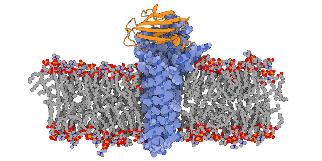
Fig.1 3X29 complex in a lipid bilayer as simulated by MemProtMD.
In this tutorial we will be working with the crystal structure of Mus musculus Claudin-19 transmembrane protein (PDB code 3X29, chain A) in complex with the unbound C-terminal fragment of the Clostridium perfringens Enteroxin (PDB code 2QUO, chain A). The PDB code of the complex is 3X29 (chains A and B).
3X29 complex is one of the cases covered in the MemCplxDB membrane protein complex benchmark (Koukos et al, 2018). Despite not being one of the most challenging cases covered in the benchmark in terms of flexibility, its relatively small size will help us describing the complete modeling protocol in the short time intended for a tutorial.
For this tutorial we will make use of the LightDock software and the LightDock server (which is currently under open beta version).
The integrative approach followed in this tutorial is described here:
- J. Roel-Touris, B. Jimenez-Garcia and A.M.J.J. Bonvin. Integrative modeling of membrane-associated protein assemblies. Nat. Commun., 11, 6210 (2020).
LightDock docking framework is described in the following publications:
-
J. Roel-Touris, A.M.J.J. Bonvin and B. Jimenez-Garcia. LightDock goes information-driven. Bioinformatics, 36:3 950-952 (2020).
-
B. Jimenez-Garcia, J. Roel-Touris, M. Romero-Durana, M. Vidal, D. Jimenez-Gonzalez, J. Fernandez-Recio. LightDock: a new multi-scale approach to protein-protein docking. Bioinformatics, 34:1 49-55 (2018).
2. General concepts
LightDock is a macromolecular docking software written in the Python programming language, designed as a framework for rapid prototyping and test of scientific hypothesis in structural biology. It was designed to be easily extensible by users and scalable for high-throughput computing (HTC). LightDock is capable of modeling backbone flexibility of molecules using anisotropic model networks (ANM) and the energetic minimization is based on the Glowworm Swarm Optimization (GSO) algorithm.
LightDock protocol is divided in two main steps: setup and simulation. On setup step, input PDB structures for receptor and ligand partners are parsed and prepared for the simulation. Moreover, a set of swarms is arranged around the receptor surface. Each of these swarms represents an independent simulation in LightDock where a fixed number of agents, called glowworms, encodes for a possible receptor-ligand pose. During the simulation step, each of these glowworms will sample a given region of the energetic landscape depending on its neighboring glowworms.
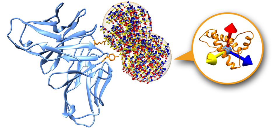
Fig.2 A receptor protein showing only two swarms. Each swarm (orange mesh sphere) contains a set of glowworms representing a possible receptor-ligand pose.
Swarms on the receptor surface can be easily filtered according to regions of interest. Figure 2 shows an example where only two swarms have been calculated to focus on two residues of interest on the receptor partner (depicted in orange). On this tutorial we will explore this capability in order to filter out incompatible transmembrane binding regions in membrane complex docking.
For more information about LightDock, please visit the tutorials section.
3. Setup/Requirements
In order to run this tutorial you will need to have the following software installed: LightDock, pdb-tools and PyMOL.
3.1. Installing LightDock
LightDock is distributed as a Python package through the Python Package Index (PyPI) repository.
3.1.1. Command line
Installing LightDock is as simple as creating a virtual environment for Python 3.6+ and running pip command (make sure your instances of virtualenv and pip are for Python 3.6+ versions). We will install the version 0.9.3.post1 of LightDock which is the latest version with support for the membrane protocol and execution in Jupyter Notebooks (see next section):
virtualenv venv
source venv/bin/activate
pip install lightdock==0.9.3.post1
If the installation finished without errors, you should be able to execute LightDock in the terminal:
lightdock3.py -v
and to see an output similar to this:
lightdock3 0.9.3.post1
3.1.2. Jupyter Notebook and Google Colab
Another option to use LightDock is through Google Colaboratory (“Colab” for short) which allows you to write and execute Python in the browser using notebooks. In case of choosing this option, simply execute in a new notebook in the first cell the following command:
!pip install lightdock==0.9.3.post1
3.2. Installing PDB-Tools
PDB-Tools is a set of Python scripts for manipulating PDB files following the philosophy of one script, one task. For different manipulating tasks on a PDB file, the procedure would be to pipe the different PDB-Tools scripts to accomplish the different tasks.
PDB-Tools is distributed as a PyPI package. To install it, simply:
pip install pdb-tools
or alternatively in a Google Colab notebook:
!pip install pdb-tools
3.3. Tutorial Notebook
We have prepared a Colab Notebook ready to be imported. Download it: tutorial.ipynb
In case of using the provided Colab notebook, go to the Colab site and upload the provided notebook (see A):
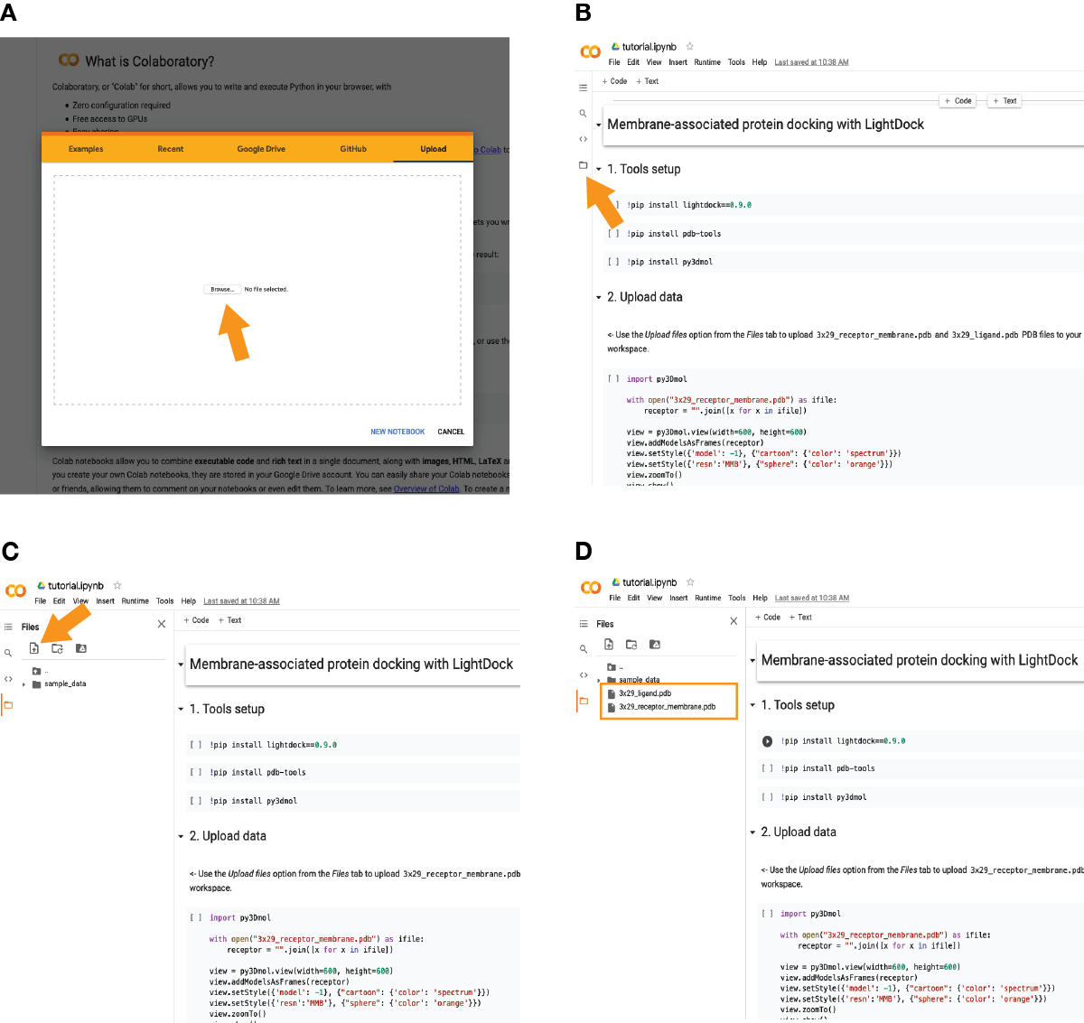
Once imported, click on the icon pointed in (B) and upload the required files as marked in (C) by the orange arrow. The two required files (3x29_receptor_membrane.pdb and 3x29_ligand.pdb) should appear now as in (D).
Then, run one by one each of the code cells as several libraries will be installed in the first code cells.
4. Data preparation
We will make use of the 3X29 complex simulated in a membrane lipid bilayer from the MemProtMD database (Newport et al., 2018).
First, browse the 3X29 complex page at MemProtMD and locate the Data Download section.
Download the PDB file corresponding to the Coarse-grained snapshot (MARTINI representation) of the 3X29 complex and rename it to 3x29_default_dppc-coarsegrained.pdb.
This file in PDB format contains the MARTINI coarse-grained (CG) representation of the phospholipid bilayer membrane and the protein complex. We will use the phosphate beads as the boundary for the transmembrane region for filtering the sampling region of interest in LightDock.
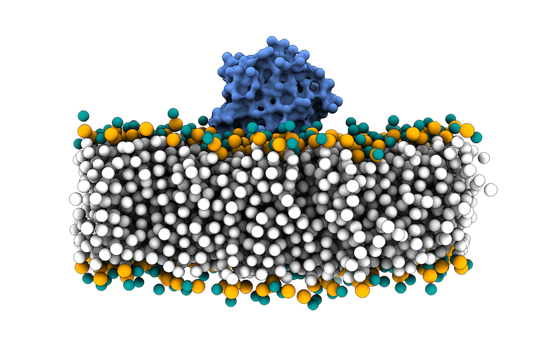
Fig.3 MARTINI Coarse-grained representation of the 3X29 complex in a lipid bilayer. Protein is depicted as blue surface, CG beads for phospholipids in white, except for NC3 beads in turquoise and PO4 beads in orange.
We have prepared a Python script to parse, rename and remove non-necessary beads for the membrane protocol in LightDock: prepare4lightdock.py. You will need to execute it in your terminal using the 3x29_default_dppc-coarsegrained.pdb PDB file as input:
python3 prepare4lightdock.py 3x29_default_dppc-coarsegrained.pdb membrane_cg.pdb
The output of this script is the membrane_cg.pdb PDB file (Figure 4).
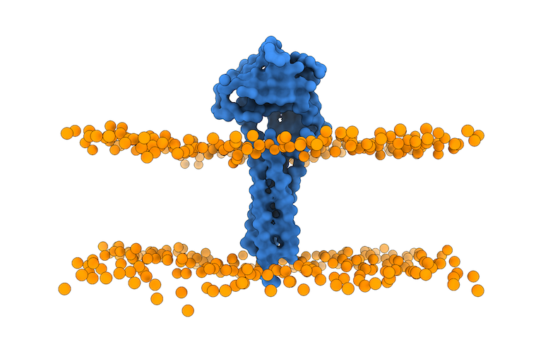
Fig.4 Lipid bilayer membrane and protein after using the `prepare4lightdock.py` script. Protein is depicted as blue surface (only CA), membrane beads ready for LightDock in orange.
The last step will be to open the just generated membrane_cg.pdb file in PyMOL to align the atomistic representation of the 3X29 receptor partner to the membrane CG bilayer:
pymol 3x29_receptor.pdb membrane_cg.pdb
Now execute the following commands on PyMOL to align the membrane with the atomistic receptor and saving the resulting PDB structure:
align 3x29_receptor and name CA, membrane_cg and name CA
remove membrane_cg and name CA
save 3x29_receptor_membrane.pdb, all
The last PyMOL command will save the aligned atomistic 3X29 receptor to the CG lipid bilayer: 3x29_receptor_membrane.pdb.
5. LightDock simulation
5.1. Simulation set up
The fist step in any LightDock simulation is setup. We will make use of lightdock3_setup.py command to initialize our 3X29 membrane simulation and the required input data is:
Use the lightdock3_setup.py command to set up the LightDock simulation:
lightdock3_setup.py 3x29_receptor_membrane.pdb 3x29_ligand.pdb --noxt --noh --membrane
In short, we are indicating to the setup command to use 3x29_receptor_membrane.pdb as the receptor partner, 3x29_ligand.pdb as the ligand, to skip NOXT and hydrogen atoms and to detect membrane beads with the --membrane flag. The output of the command should look similar to this:
[lightdock3_setup] INFO: Ignoring OXT atoms
[lightdock3_setup] INFO: Ignoring Hydrogen atoms
[lightdock3_setup] INFO: Reading structure from 3x29_receptor_membrane.pdb PDB file...
[pdb] WARNING: Possible problem: [SideChainError] Incomplete sidechain for residue GLN.61
[pdb] WARNING: Possible problem: [SideChainError] Incomplete sidechain for residue GLN.63
[pdb] WARNING: Possible problem: [SideChainError] Incomplete sidechain for residue LYS.65
[pdb] WARNING: Possible problem: [SideChainError] Incomplete sidechain for residue LEU.66
[pdb] WARNING: Possible problem: [SideChainError] Incomplete sidechain for residue ASP.68
[pdb] WARNING: Possible problem: [SideChainError] Incomplete sidechain for residue HIS.76
[pdb] WARNING: Possible problem: [SideChainError] Incomplete sidechain for residue MET.95
[pdb] WARNING: Possible problem: [SideChainError] Incomplete sidechain for residue MET.102
[pdb] WARNING: Possible problem: [SideChainError] Incomplete sidechain for residue LYS.103
[pdb] WARNING: Possible problem: [SideChainError] Incomplete sidechain for residue LYS.115
[pdb] WARNING: Possible problem: [SideChainError] Incomplete sidechain for residue ARG.117
[lightdock3_setup] INFO: 1608 atoms, 601 residues read.
[lightdock3_setup] INFO: Ignoring OXT atoms
[lightdock3_setup] INFO: Ignoring Hydrogen atoms
[lightdock3_setup] INFO: Reading structure from 3x29_ligand.pdb PDB file...
[lightdock3_setup] INFO: 933 atoms, 117 residues read.
[lightdock3_setup] INFO: Calculating reference points for receptor 3x29_receptor_membrane.pdb...
[lightdock3_setup] INFO: Reference points for receptor found, skipping
[lightdock3_setup] INFO: Done.
[lightdock3_setup] INFO: Calculating reference points for ligand 3x29_ligand.pdb...
[lightdock3_setup] INFO: Reference points for ligand found, skipping
[lightdock3_setup] INFO: Done.
[lightdock3_setup] INFO: Saving processed structure to PDB file...
[lightdock3_setup] INFO: Done.
[lightdock3_setup] INFO: Saving processed structure to PDB file...
[lightdock3_setup] INFO: Done.
[lightdock3_setup] INFO: Calculating starting positions...
[lightdock3_setup] INFO: Generated 62 positions files
[lightdock3_setup] INFO: Done.
[lightdock3_setup] INFO: Number of calculated swarms is 62
[lightdock3_setup] INFO: Preparing environment
[lightdock3_setup] INFO: Done.
[lightdock3_setup] INFO: LightDock setup OK
In previous versions of LightDock, the number of swarms of the simulated was given by the user (typically around 400), but since version 0.9.0, the number of swarms of the simulation is automatically calculated depending on the surface area of the receptor structure. However, the number of swarms can be fixed by the user using the -s flag for reproducibility of old results purpose. Another difference with previous versions is that the number of glowworms is now default to 200. This value has been extensively tested on our previous work, but it may be defined by the user as well using the -g flag.
A complete list of the lightdock3_setup.py command options might be obtained executing the command without arguments or with the --help flag:
usage: lightdock3_setup [-h] [-s SWARMS] [-g GLOWWORMS] [--seed_points STARTING_POINTS_SEED] [--noxt] [--noh] [--verbose_parser] [-anm] [--seed_anm ANM_SEED] [-ar ANM_REC]
                        [-al ANM_LIG] [-r restraints] [-membrane] [-transmembrane]
                        [-sp] [-sd SURFACE_DENSITY] [-sr SWARM_RADIUS]
                        receptor_pdb_file ligand_pdb_file
lightdock3_setup: error: the following arguments are required: receptor_pdb_file, ligand_pdb_file
The setup command has generated several files and directories:
Question: What is the content of the setup.json file?
Question: What does the init directory contain?
We may visualize the distribution of swarms over the receptor:
pymol lightdock_3x29_receptor_membrane.pdb init/swarm_centers.pdb
Fig.5 Distribution of swarms in the current simulation.
Question: Is this a rigid-body or a flexible simulation?
5.2. Running the simulation
The simulation is ready to run at this point. The number of swarms after focusing on the extramembranous region of the membrane protein is of 62.
LightDock optimization strategy (using the GSO algorithm) is agnostic of the scoring function (force-field). There are several scoring functions available at LightDock, from atomistic to coarse-grained. In this tutorial we will make use of fastdfire, which is the implementation of DFIRE using the Python C API and the default one if no scoring function is specified by the user. Find here a complete list of the current supported scoring functions by LightDock.
Simulation is the most time-consuming part of the protocol. For that reason, we will only simulate one of the 62 total swarms. Pick a swarm number between [0..61] and use that id in the -l argument:
lightdock3.py setup.json 100 -c 1 -s fastdfire -l 60
In the command above, we specify the JSON file of the simulation (setup.json), the number of steps of the simulation (100), the number of CPU cores to use (-c 1), the scoring function (-s fastdfire). If no -l argument is provided, the protocol would simulate all the swarms.
For your convenience, you can download the full run as a compressed zip file (45MB).
Once the simulation has finished, navigate to the swarm_60 directory (or the one you have selected) and list the directory.
Question: How many gso_* files have been generated? Which one corresponds to the last step of the simulation?
5.3. Generating models
Once the simulation has finished successfully, it is time to generate the predicted models. For each swarm, there is a gso_100.out file containing the information to generate as many models as glowworms were defined in the simulation (200 in this tutorial). The command in charge of generating the models is lgd_generate_conformations.py.
Pick a swarm folder and generate the 200 models simulated as in step 100:
lgd_generate_conformations.py 3x29_receptor_membrane.pdb 3x29_ligand.pdb swarm_60/gso_100.out 200
You should see an output similar to this:
[generate_conformations] INFO: Reading ../lightdock_3x29_receptor_membrane.pdb receptor PDB file...
[pdb] WARNING: Possible problem: [SideChainError] Incomplete sidechain for residue GLN.61
[pdb] WARNING: Possible problem: [SideChainError] Incomplete sidechain for residue GLN.63
[pdb] WARNING: Possible problem: [SideChainError] Incomplete sidechain for residue LYS.65
[pdb] WARNING: Possible problem: [SideChainError] Incomplete sidechain for residue LEU.66
[pdb] WARNING: Possible problem: [SideChainError] Incomplete sidechain for residue ASP.68
[pdb] WARNING: Possible problem: [SideChainError] Incomplete sidechain for residue HIS.76
[pdb] WARNING: Possible problem: [SideChainError] Incomplete sidechain for residue MET.95
[pdb] WARNING: Possible problem: [SideChainError] Incomplete sidechain for residue MET.102
[pdb] WARNING: Possible problem: [SideChainError] Incomplete sidechain for residue LYS.103
[pdb] WARNING: Possible problem: [SideChainError] Incomplete sidechain for residue LYS.115
[pdb] WARNING: Possible problem: [SideChainError] Incomplete sidechain for residue ARG.117
[generate_conformations] INFO: 1608 atoms, 601 residues read.
[generate_conformations] INFO: Reading ../lightdock_3x29_ligand.pdb ligand PDB file...
[generate_conformations] INFO: 933 atoms, 117 residues read.
[generate_conformations] INFO: Read 200 coordinate lines
[generate_conformations] INFO: Generated 200 conformations
5.4. Clustering models
To remove very similar and redundant models in the same swarm, we will cluster the 200 generated models:
lgd_cluster_bsas.py swarm_60/gso_100.out
After a verbose output of the command above, a new file cluster.repr is generated inside the swarm_60 folder. This file should look like this:
0:3:26.80832:115:lightdock_115.pdb
1:9:24.45152:42:lightdock_42.pdb
2:62:22.70320:37:lightdock_37.pdb
3:35:20.35832:0:lightdock_0.pdb
4:41:16.69347:38:lightdock_38.pdb
5:3:15.71026:79:lightdock_79.pdb
6:7:13.89057:72:lightdock_72.pdb
7:7:11.84427:164:lightdock_164.pdb
8:1:8.69611:92:lightdock_92.pdb
9:1:2.92199:137:lightdock_137.pdb
10:22:-0.00771:95:lightdock_95.pdb
11:2:-24.59441:93:lightdock_93.pdb
12:7:-31.35821:57:lightdock_57.pdb
Each line represents a different cluster and lines are sorted from best to worst energy. For each line, there is information about the cluster id, the number of structures in the cluster, the best energy of the cluster, the glowworm id of the model with best energy and the PDB file name of the structure with best energy.
Open the best predicted model for this swarm in PyMOL and have a look.
pymol swarm_60/lightdock_115.pdb
Question: How does this model look in general? What about the side chains?
6. Analysis
In the CAPRI (Critical Prediction of Interactions) Méndez et al. 2003 experiment, one of the parameters used is the Ligand root-mean-square deviation (L-RMSD) which is calculated by superimposing the structures onto the backbone atoms of the receptor and calculating the RMSD on the backbone residues of the ligand. To calculate the L-RMSD it is possible to either use the software Profit or Pymol.
We will have a quick look at the top 10 models predicted by LightDock and compare them with the 3X29 complex reference. Below you will find a table with the top 10 models according to the LightDock ranking (click on a name to download):
| Top | Docking (LightDock) |
|---|---|
| 1 | swarm_22_112.pdb |
| 2 | swarm_37_11.pdb |
| 3 | swarm_39_11.pdb |
| 4 | swarm_60_115.pdb |
| 5 | swarm_54_167.pdb |
| 6 | swarm_37_34.pdb |
| 7 | swarm_55_181.pdb |
| 8 | swarm_60_42.pdb |
| 9 | swarm_37_169.pdb |
| 10 | swarm_37_83.pdb |
You can also download as compressed files:
6.1. Visualizing and aligning in PyMOL
First, open the target and reference structures in PyMOL (in this case top 1 from LightDock ranking):
pymol swarm_22_112.pdb 3x29_reference.pdb
Color by chain (and leave orange the membrane beads):
util.cbc
color orange, swarm_22_112 and name BJ
Align both structures to the receptor partner (chain A):
align swarm_22_112 and chain A, 3x29_reference and chain A
Center visualization:
z vis
6.2. Calculating L-RMSD in PyMOL
From the alignment of the previous section, we can easily calculate the L-RMSD in PyMOL:
First, remove all segid information to let PyMOL correctly find the target chains:
alter all, segi = ' '
And now calculate L-RMSD using rms_cur command:
rms_cur swarm_22_112 and chain B, 3x29_reference and chain B
Which leaves a L-RMSD of 22.7Å.
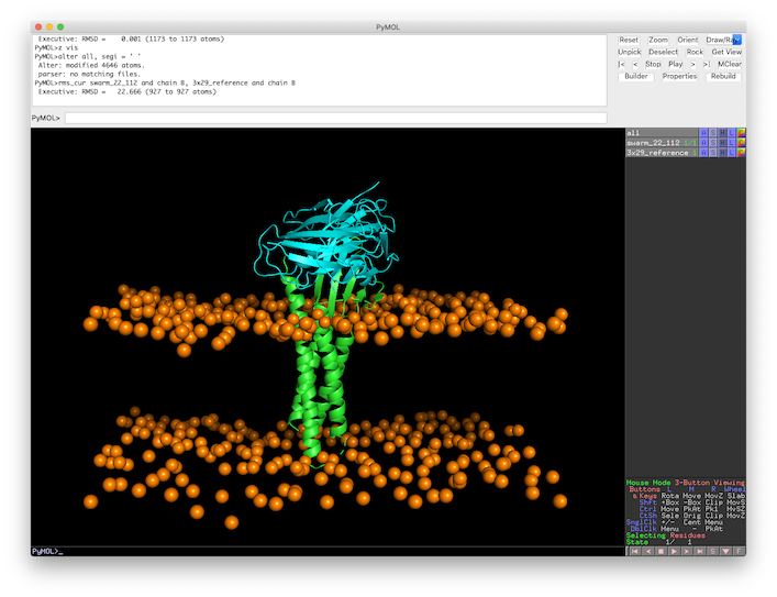
Fig.6 L-RMSD calculation in PyMOL of the top 1 model against the 3X29 reference structure.
Repeat the same process for more structure on the top 10 ranking from LightDock
See the calculated L-RMSDs:
swarm_22_112.pdb 22.551Å
swarm_37_11.pdb 11.850Å
swarm_39_11.pdb 13.424Å
swarm_60_115.pdb 5.735Å
swarm_54_167.pdb 25.031Å
swarm_37_34.pdb 28.587Å
swarm_55_181.pdb 20.470Å
swarm_60_42.pdb 10.801Å
swarm_37_169.pdb 14.894Å
swarm_37_83.pdb 25.857Å
Question: Which is the best structure in terms of L-RMSD in the LightDock ranking?
In CAPRI, the L-RMSD value defines the quality of a model:
- incorrect model: L-RMSD>10Å
- acceptable model: L-RMSD<10Å
- medium quality model: L-RMSD<5Å
- high quality model: L-RMSD<1Å
Question: What is the quality of these models? Did any model pass the acceptable threshold?
7. What if membrane information is not available?
In case there is no membrane simulated in the MemProtMD database, we can still generate an approximated version using the Membrane Builder online tool (a.k.a. Membranator).
Go to Membrane Builder and use 3x29_receptor.pdb structure in the form and pick a residue which will be the boundary of the artificial coarse-grained generated membrane (in the form is called Anchor residue). In Figure 7 we selected residue A.LEU.50, but go check the UniProt entry for this protein.
Question: A better anchor residue might be A.LEU.27. Why?
You may leave the rest of the fields as default.
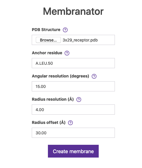
Fig.7 The Membrane builder online tool.
Click on Create membrane and wait for the output (similar to figure 8).
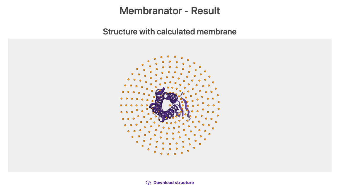
Fig.8 Generated membrane by the Membrane builder online tool.
Click on the Download structure link and save the PDB structure (by default is called result.pdb, you may rename it to 3x29_receptor_membranator.pdb).
Question: Why is there a central bead in the generated membrane?
At this point, you may go back to section 5 and repeat the simulation but using this new structure as the receptor. A different approach could be to use the Lightdock server.
Using the LightDock server is really easy and it does not require registration for quick tests, but blind docking is only available upon registration. Nonetheless, we have prepared a simulation for you.
Download the results and have a look at the top directory
Question: Do you observe differences between the top structures of this simulation compared to the previous one on this tutorial? (Hint: see next section)
8. Bonus track: refinement
LightDock can perform rigid-body docking (by default) or include flexibility of the backbone through the Anisotropic Network Model if activated (anm flag). In both scenarios, the scoring function helps removing high-clashing poses from the prediction pool, but this does not guarantee an optimal packing of side-chains or few clashes. A common strategy to avoid these inaccuracies is to refine the top predicted structures.
In our work Integrative modeling of membrane-associated protein assemblies, the top predicted structures by LightDock were further refined using the well-known HADDOCK web server. In a twin tutorial, we describe step by step the refinement protocol for removing clashes at the interface of protein complexes in HADDOCK. You can learn more about the HADDOCK software and all its applications at the official education site.
In the LightDock server, we have added an extra step to perform a quick relaxation molecular dynamics simulation for the top 5 or top 10 predicted structures by LightDock. The amazing OpenMM toolkit is used for this purpose.
9. Conclusions
We have demonstrated an integrative modeling protocol for membrane-associated protein assemblies that accounts for the topological information provided by the membrane in the modeling process.
In general, some knowledge of the putative binding interface is known to help the modeling of biomolecular interactions, often allowing to generate more accurate models.
It is of paramount importance not to blindly trust docking predictions and rankings. Always inspect the results and predictions and further assess their quality using more metrics and validate your results (if possible) agains experimental data.