Complex protein-protein docking with restraints
This is a complete example of the LightDock docking protocol to model the 4G6M protein complex with the use of residue restraints.
IMPORTANT Please, make sure that you have the python3 version of LightDock installed (pip3 install lightdock). We advise you to follow the basic tutorial about how to run a quick LightDock simulation
Copying the data
Create a directory and copy the sample data provided.
cd Desktop
mkdir test
cd test
curl -O https://raw.githubusercontent.com/lightdock/lightdock.github.io/master/tutorials/examples/4G6M/4G6M_rec.pdb
curl -O https://raw.githubusercontent.com/lightdock/lightdock.github.io/master/tutorials/examples/4G6M/4G6M_lig.pdb
Specifying residue restraints
LightDock is able to use information derived from either experimental information and/or bioinformatic predictions to drive the docking at several levels. This information is used in the form of residue restraints.
To do so, we first need to create a restraints.list file of the following form.
R A.GLN.27
R A.SER.30
R A.TYR.32
...
L B.SER.68
L B.CYS.69
L B.VAL.70
...
Where the first column will indicate whether it is a receptor R or ligand L restraint, followed by CHAIN_ID.RESIDUE_NAME.RESIDUE_NUMBER. In this case, LightDock will consider these residue restraints as ACTIVE.
By contrast, if you want to define your residue restraints as PASSIVE you should add an additional column with a P label.
R A.GLN.27 P
R A.SER.30 P
R A.TYR.32 P
...
L B.SER.68 P
L B.CYS.69 P
L B.VAL.70 P
...
NOTE For a detailed description of the exact implications of ACTIVE and PASSIVE restraints in LightDock, please refer to LightDock goes information-driven
For the sake of simplicity, we will use a list of residue restraints already formatted.
curl -O https://raw.githubusercontent.com/lightdock/lightdock.github.io/master/tutorials/examples/4G6M/restraints.list
Setup
First, we need to run the setup step. We will specify a number of 400 initial swarms and 200 glowworms. We will also enable flexibility, exclude the terminal oxygens and ALL hydrogens (not parametrized in fastdfire scoring function).
At this step, we need to also specify the residue restraints that will bias the docking simulation.
lightdock3_setup.py 4G6M_rec.pdb 4G6M_lig.pdb 400 200 -anm --noxt --noh -rst restraints.list

@> ProDy is configured: verbosity='info'
[lightdock_setup] INFO: Reading structure from 4G6M_rec.pdb PDB file...
[lightdock_setup] INFO: 1782 atoms, 230 residues read.
[lightdock_setup] INFO: Reading structure from 4G6M_lig.pdb PDB file...
[lightdock_setup] INFO: 1194 atoms, 149 residues read.
[lightdock_setup] INFO: Calculating reference points for receptor 4G6M_rec.pdb...
[lightdock_setup] INFO: Done.
[lightdock_setup] INFO: Calculating reference points for ligand 4G6M_lig.pdb...
[lightdock_setup] INFO: Done.
[lightdock_setup] INFO: Saving processed structure to PDB file...
[lightdock_setup] INFO: Done.
[lightdock_setup] INFO: Saving processed structure to PDB file...
[lightdock_setup] INFO: Done.
[lightdock_setup] INFO: 10 normal modes calculated
[lightdock_setup] INFO: 10 normal modes calculated
[lightdock_setup] INFO: Reading restraints from restraints.list
[lightdock_setup] INFO: Number of receptor restraints is: 20 (active), 0 (passive)
[lightdock_setup] INFO: Number of ligand restraints is: 21 (active), 0 (passive)
[lightdock_setup] INFO: Calculating starting positions...
[lightdock_setup] INFO: Generated 84 positions files
[lightdock_setup] INFO: Done.
[lightdock_setup] INFO: Number of swarms is 84 after applying restraints
[lightdock_setup] INFO: Preparing environment
[lightdock_setup] INFO: Done.
[lightdock_setup] INFO: LightDock setup OK
At first glance, we see that the initial number of specified swarms (400) has been reduced to 84. This means that the sampling will be targeted towards a desired area of the receptor.
Moreover, since we have also specified residue restraints on the ligand, the initial glowworm conformations have been oriented so that those residues will be facing the desired receptor’s region.
Please refer to the following picture for a graphical description of the setup.
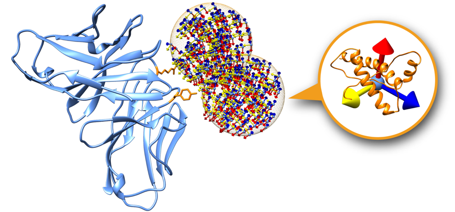
This is a representation of two swarms (orange mesh) over the surface of the 4G6M_rec.pdb (blue). In orange, two residues considered as restraints and therefore used to filter out the initial swarms prior the simulation. The initial orientations of the ligands within the swarms are represented using an orthogonal axis (x, y, z).
Simulation
We can run our simulation in a local machine or in a HPC cluster. For the first option, simply run the following command.
lightdock3.py setup.json 100 -s fastdfire -c 8
Where the flag -c 8 indicates LightDock to use 8 available cores. For this example we will run 100 steps of the protocol and the C implementation of the DFIRE function -s fastdfire.
To run a LightDock job on a HPC cluster, a Portable Batch System (PBS) file can be generated. This PBS file defines the commands and cluster resources used for the job. A PBS file is a plain-text file that can be easily edited with any UNIX editor.
For example, create a submit_job.sh file containing:
#PBS -N LightDock-4G6M
#PBS -q medium
#PBS -l nodes=1:ppn=16
#PBS -S /bin/bash
#PBS -d ./
#PBS -e ./lightdock.err
#PBS -o ./lightdock.out

lightdock3.py setup.json 100 -s fastdfire -c 16
This script tells the PBS queue manager to use 16 cores of a single node in a queue with name medium, with job name LigthDock-4G6M and with standard output to lightdock.out and error output redirected to lightdock.err.
To run this script you can do it as:
qsub < submit_job.sh
Analysis
Once the simulation has finished (it takes around 1-2 min per 10 steps per swarm), we need to analyze the results as:
- (1) Generate the structures per swarm (200 glowworms per swarm in this example)
- (2) Clusterize the predictions per swarm
- (3) Generate the ranking files
- (4) Filter by a percentage of satisfied restraints (this is a highly recommended step: >40% in this example)
Here there is a PBS script to do so.
#PBS -N 4G6M-anal
#PBS -q medium
#PBS -l nodes=1:ppn=8
#PBS -S /bin/bash
#PBS -d ./
#PBS -e ./analysis.err
#PBS -o ./analysis.out

### Calculate the number of swarms ###

s=`ls -d ./swarm_* | wc -l`
swarms=$((s-1))


### Create files for Ant-Thony ###

for i in $(seq 0 $swarms)
  do
    echo "cd swarm_${i}; lgd_generate_conformations.py ../4G6M_rec.pdb ../4G6M_lig.pdb  gso_100.out 200 > /dev/null 2> /dev/null;" >> generate_lightdock.list;
  done

for i in $(seq 0 $swarms)
  do
    echo "cd swarm_${i}; lgd_cluster_bsas.py gso_100.out > /dev/null 2> /dev/null;" >> cluster_lightdock.list;
  done


### Generate LightDock models ###

ant_thony.py -c 8 generate_lightdock.list;


### Clustering BSAS (rmsd) within swarm ###

ant_thony.py -c 8 cluster_lightdock.list;


### Generate ranking files for filtering ###

lgd_rank.py $s 100;


### Filtering models by >40% of satisfied restraints ###

lgd_filter_restraints.py --cutoff 5.0 --fnat 0.4 rank_by_scoring.list restraints.list A B > /dev/null 2> /dev/null;
NOTE You can also run the previous commands locally in a sequential way.
Once the analysis is finished, a new folder called filtered has been created, which contains any predicted structure which satisfies our 40% filtering. Inside of this directory, there is a file with the ranking of these structures by LightDock DFIRE (fastdfire) score (the more positive the better) rank_filtered.list.
We provide for this example a compressed filtered folder filtered.tgz which contains (when decompressed) a ranking lgd_filtered_rank.list file.
For all the filtered structures, interface RMSD (i-RMSD), ligand RMSD (l-RMSD) and fraction of native contacts (fnc) according to CAPRI criteria have been calculated.
head lgd_filtered_rank.list
# structure    		i-RMSD  l-RMSD  fnc      	Score
swarm_83_154.pdb	2.091	2.012	0.603448	56.869
swarm_50_151.pdb	3.082	4.001	0.327586	50.536
swarm_7_192.pdb	        1.553	1.461	0.586207	48.936
swarm_36_168.pdb	1.132	1.385	0.827586	48.870
swarm_48_19.pdb	        3.687	4.205	0.258621	48.739
swarm_11_136.pdb	2.231	2.390	0.448276	48.662
swarm_52_171.pdb	3.933	4.052	0.155172	47.808
swarm_49_183.pdb	3.589	3.775	0.258621	47.659
swarm_48_49.pdb	        1.562	2.100	0.793103	47.234
swarm_65_93.pdb	        1.282	1.130	0.844828	45.372
As you may observe, by using this specific information, LightDock is able to generate very high quality models. Some of them sharing >60% of contacts as compared to the crystal structure.
References
For a more complete description of the algorithm as well as different tutorials, please refer to LightDock, or check the following references:
-
Integrative Modeling of Membrane-associated Protein Assemblies
Jorge Roel-Touris, Brian Jiménez-García & Alexandre M.J.J. Bonvin
Nat Commun 11, 6210 (2020); doi: https://doi.org/10.1038/s41467-020-20076-5 -
LightDock goes information-driven
Jorge Roel-Touris, Alexandre M.J.J. Bonvin and Brian Jiménez-García
Bioinformatics, Volume 36, Issue 3, 1 February 2020, Pages 950–952, doi: https://doi.org/10.1093/bioinformatics/btz642 -
LightDock: a new multi-scale approach to protein–protein docking
Brian Jiménez-García, Jorge Roel-Touris, Miguel Romero-Durana, Miquel Vidal, Daniel Jiménez-González and Juan Fernández-Recio
Bioinformatics, Volume 34, Issue 1, 1 January 2018, Pages 49–55, doi: https://doi.org/10.1093/bioinformatics/btx555